DIP
Exp-1: Study of MATLAB software and its basic commands.
MATLAB (Matrix Laboratory) is a high-level programming language and environment used primarily for numerical computing, data analysis, algorithm development, and visualization. It is widely used in academia and industry for tasks involving mathematics, engineering, and scientific computations.
Key Features of MATLAB:
1. Interactive Environment: MATLAB provides an interactive platform to execute commands and visualize data.
2. Matrix Operations: Built-in support for matrix and array mathematics.
3. Rich Visualization: Easy-to-use functions for plotting and visualizing data.
4. Extensive Toolboxes: Additional toolboxes are available for various applications (e.g., Signal Processing, Image Processing, Machine Learning).
5. Cross-Platform: MATLAB runs on Windows, macOS, and Linux.
Basic Commands in MATLAB
1. Variable Assignment
x = 10; % Assigns the value 10 to variable x y = 5; % Assigns the value 5 to variable y
2. Arithmetic Operations
sum = x + y; % Addition difference = x - y; % Subtraction product = x * y; % Multiplication quotient = x / y; % Division
power = x^2; % Exponentiation (x squared)
3. Creating Matrices and Vectors
A = [1, 2; 3, 4]; % 2x2 matrix
B = [5, 6; 7, 8]; % Another 2x2 matrix
C = [1, 2, 3, 4, 5]; % Row vector
D = [1; 2; 3; 4; 5]; % Column vector
4. Matrix Operations
C_sum = A + B; % Matrix addition
C_diff = A - B; % Matrix subtraction C_product = A * B; % Matrix multiplication C_transpose = A'; % Transpose of matrix A C_inverse = inv(A); % Inverse of matrix A
5. Accessing Elements
element = A(1, 2); % Access element at row 1, column 2 row_vector = A(1, :); % Access all elements in row 1 column_vector = A(:, 2); % Access all elements in column 2
6. Basic Functions
mean_value = mean(A(:)); % Calculate mean of all elements in A
std_dev = std(A(:)); % Calculate standard deviation of elements in A max_value = max(A); % Find the maximum value in A
7. Plotting
x = 0:0.1:10; % Create x values from 0 to 10 with a step of 0.1 y = sin(x); % Compute y values as the sine of x
figure; % Create a new figure window
plot(x, y); % Create a 2D plot xlabel('x-axis'); % Label for x-axis ylabel('y = sin(x)'); % Label for y-axis title('Sine Wave'); % Title of the plot
grid on; % Display grid on the plot
8. Control Flow
% If-Else Statement if x > 5
disp('x is greater than 5');
else end
disp('x is less than or equal to 5');
% For Loop
for i = 1:5
disp(['Iteration: ', num2str(i)]);
end
% While Loop count = 1; while count <= 5
disp(['Count: ', num2str(count)]); count = count + 1; % Increment count
end
9. Functions
% Define a simple function function output = square(num)
output = num^2; % Square the input number
end
% Call the function
result = square(4); % result will be 16
Conclusion
MATLAB is a powerful tool for engineers and scientists. Understanding its basic commands is essential for effectively using the software. These basic commands provide a foundation for using MATLAB effectively. Familiarizing ourself with these commands will help you perform a wide range of numerical and graphical tasks in MATLAB.
Exp 2: Write a program to generate and modify matrices using standard commands in MATLAB.
Code:-
% Step 1: Create a 2x2 matrix
A = [1 2; 3 4];
disp('Matrix A:');
disp(A);
% Step 2: Change an element (1st row, 1st column)
A(1, 1) = 10;
disp('Matrix A after modification:');
disp(A);
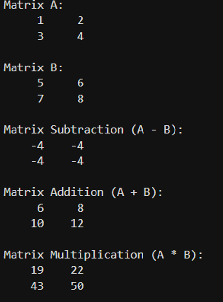
Exp 3: Write a program to perform matrix operations in MATLAB.
Code:-
% Create two 2x2 matrices
A = [1 2; 3 4];
B = [5 6; 7 8];
disp('Matrix A:');
disp(A);
disp('Matrix B:');
disp(B);
% Subtract the matrices
C = A - B;
disp('Matrix Subtraction (A - B):');
disp(C);
% Matrix Addition
D = A + B;
disp('Matrix Addition (A + B):');
disp(D);
% Matrix Multiplication
E = A * B;
disp('Matrix Multiplication (A * B):');
disp(E);
Output: -
Exp 4: write a program to generate plot using MATLAB.
Code: -
% Create x and y data
x = 0:0.1:10;
y = sin(x);
% Generate the plot
plot (x, y);
>> % Create x and y data
x = 0:0.1:10;
y = sin(x);
% Generate the plot
plot (x, y);
% Add labels
xlabel('x');
ylabel('sin(x)');
Output:-
Exp 5: Write a program to read an image, convert it in grayscale and black & white image, show image in MATLAB.
Code:-
% Step 1: Read the image
img = imread('Screenshot 2024-11-29 at 11.39.21 AM.jpeg');
% Step 2: Convert the image to grayscale
gray_img = rgb2gray(img);
% Step 3: Convert the image to black and white (binary image)
bw_img = imbinarize(gray_img);
% Step 4: Display the original, grayscale, and black & white images
figure;
imshow(img);
title('Original Image');
figure;
imshow(gray_img);
title('Grayscale Image');
figure;
imshow(bw_img);
title('Black & White Image');
Output:-
Exp 6: Write a program to perform various mathematical operations on image in MATLAB.
Code:-
% Load the image
image = imread('Screenshot 2024-11-29 at 11.39.21 AM.jpeg'); % Replace with your image file
grayImage = rgb2gray(image); % Convert to grayscale for simplicity
% Display the original image
figure;
subplot(2,3,1);
imshow(grayImage);
title('Original Image');
% Brightness Adjustment
brightImage = grayImage + 50; % Increase brightness by adding constant value
subplot(2,3,2);
imshow(brightImage);
title('Brightness Adjusted');
% Contrast Enhancement
contrastImage = imadjust(grayImage, [0.3 0.7], [0 1]); % Enhance contrast
subplot(2,3,3);
imshow(contrastImage);
title('Contrast Enhanced');
% Edge Detection
edgeImage = edge(grayImage, 'Sobel'); % Apply Sobel edge detection
subplot(2,3,4);
imshow(edgeImage);
title('Edge Detection');
% Image Negation
negativeImage = 255 - grayImage; % Subtract pixel values from 255
subplot(2,3,5);
imshow(negativeImage);
title('Negative Image');
% Image Blurring (using Gaussian filter)
h = fspecial('gaussian', [5 5], 2); % Gaussian filter
blurredImage = imfilter(grayImage, h, 'replicate');
subplot(2,3,6);
imshow(blurredImage);
title('Blurred Image');
Output:-
Exp 7: Write a program to find image negative in MATLAB.
Code:-
% Step 1: Read the original image
img = imread('Screenshot 2024-11-29 at 11.39.21 AM.jpeg');
% Step 2: Convert to grayscale if the image is colored
if size(img, 3) == 3
img = rgb2gray(img); % Convert RGB to grayscale
end
% Step 3: Find the negative of the image
negative_img = 255 - img; % Subtract pixel values from 255
% Step 4: Display the original and negative images
figure;
% Original Image
imshow(img);
title('Original Image');
% Negative Image
figure;
imshow(negative_img);
title('Negative Image');
output:-
Exp 8: Apply power law transformation for following image. Analyse result.
Code:-
% Step 1: Read the original image
img = imread('Screenshot 2024-11-29 at 11.39.21 AM.jpeg');
% Step 2: Convert to grayscale if the image is colored
if size(img, 3) == 3
img = rgb2gray(img); % Convert RGB to grayscale
end
% Step 3: Normalize the image to the range [0, 1]
img_normalized = double(img) / 255;
% Step 4: Apply Power-Law Transformation
c = 1; % Constant value
gamma = 2; % Change this value to adjust brightness (e.g., 0.5, 1, 2)
transformed_img = c * (img_normalized .^ gamma); % Power-law transformation
% Correct: Normalize the result to [0, 1] before scaling
transformed_img = mat2gray(transformed_img); % Normalize
% Step 5: Convert the transformed image back to uint8
transformed_img = uint8(transformed_img * 255); % Scale back to [0, 255]
% Step 6: Display the original and transformed images
figure;
% Original Image
imshow(img);
title('Original Image');
% Transformed Image
figure;
imshow(transformed_img);
title('Power-Law Transformed Image (gamma = 2)');
Output:-
Analyzing the Result:
· Effect of Gamma:
· A gamma value of less than 1 (e.g., 0.5) will brighten the image, especially the darker regions, which can help in enhancing details in shadowed areas.
· A gamma value greater than 1 (e.g., 2) will darken the image, enhancing the bright areas, which can lead to better contrast in images with significant brightness variation.
Exp- 9 : Write MatLab code to plot histogram of a image and apply histogram equalization on the same image.
Code:-
% Reading the image
image = imread('Screenshot 2024-11-29 at 11.39.21 AM.jpeg');
image = rgb2gray(image); % Convert to grayscale if it's a color image
% Plotting original image and its histogram figure;
% Displaying the original image subplot(2,2,1);
imshow(image); title('Original Image');
% Displaying the histogram of the original image subplot(2,2,2);
imhist(image);
title('Histogram of Original Image');
% Applying histogram equalization equalizedImage = histeq(image);
% Displaying the histogram-equalized image subplot(2,2,3);
imshow(equalizedImage); title('Histogram Equalized Image');
% Displaying the histogram of the equalized image subplot(2,2,4);
imhist(equalizedImage); title('Histogram of Equalized Image');
Output:-
Exp 10: Apply different size averaging filter on an Image and compare results.
Code:-
% Reading the image
image = imread('Screenshot 2024-11-29 at 11.39.21 AM.jpeg');
image = rgb2gray(image); % Convert to grayscale if it's a color image
% Define filter sizes
filterSizes = [3, 5, 7];
% Displaying original and first filtered image on first page with larger figure
figure(1);
set(gcf, 'Position', get(0, 'Screensize')); % Set figure to full screen
subplot(1,2,1);
imshow(image, 'InitialMagnification', 'fit'); % Display original image
title('Original Image', 'FontSize', 14); % Increase title font size
% Applying and displaying the first filter size
h = fspecial('average', filterSizes(1));
filteredImage1 = imfilter(image, h, 'replicate');
subplot(1,2,2);
imshow(filteredImage1, 'InitialMagnification', 'fit');
title([num2str(filterSizes(1)) 'x' num2str(filterSizes(1)) ' Filter'], 'FontSize', 14);
% Displaying the next two filtered images on the second page
figure(2);
set(gcf, 'Position', get(0, 'Screensize')); % Set figure to full screen
% Applying and displaying the second filter size
subplot(1,2,1);
h = fspecial('average', filterSizes(2));
filteredImage2 = imfilter(image, h, 'replicate'); imshow(filteredImage2, 'InitialMagnification', 'fit');
title([num2str(filterSizes(2)) 'x' num2str(filterSizes(2)) ' Filter'], 'FontSize', 14);
% Applying and displaying the third filter size subplot(1,2,2);
h = fspecial('average', filterSizes(3)); filteredImage3 = imfilter(image, h, 'replicate');
imshow(filteredImage3, 'InitialMagnification', 'fit');
title([num2str(filterSizes(3)) 'x' num2str(filterSizes(3)) ' Filter'], 'FontSize', 14);
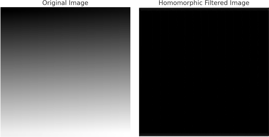
Exp 11: Apply homomorphic filtering on any appropriate image
Code:-
% Load and convert the image to grayscale
img = imread('Screenshot 2024-11-29 at 11.39.21 AM.jpeg'); % Replace with your image file
if size(img, 3) == 3
img = rgb2gray(img); % Convert to grayscale if it's a color image
end
img = im2double(img); % Convert to double for processing
% Perform logarithmic transformation
logImage = log(1 + img);
% Design a high-pass Butterworth filter for frequency domain
[M, N] = size(img);
[u, v] = meshgrid(1:N, 1:M);
u = u - ceil(N/2);
v = v - ceil(M/2);
D = sqrt(u.^2 + v.^2);
D0 = 30; % Cutoff frequency
n = 2; % Order of the filter
H = 1 ./ (1 + (D0 ./ (D + eps)).^(2 * n)); % High-pass Butterworth filter
H = fftshift(H); % Center the filter
% Perform FFT on the logarithmic image
FFTImage = fft2(logImage);
% Apply the filter
FilteredFFTImage = H .* FFTImage;
% Perform inverse FFT and exponential transformation
FilteredImage = real(ifft2(FilteredFFTImage));
FilteredImage = exp(FilteredImage) - 1;
% Normalize the output image for display
FilteredImage = mat2gray(FilteredImage);
% Display results
figure;
subplot(1, 2, 1);
imshow(img);
title('Original Image');
subplot(1, 2, 2);
imshow(FilteredImage);
title('Homomorphic Filtered Image');
Output:-


Comments
Post a Comment